Forecast Step 129

The first 128 forecast steps can be correct while the next 128 violate the same invariant. A patch-based decoder makes that possible: the initial output and the autoregressive continuation travel through different branches.

TimesFM's force_flip_invariance option gives a precise property to test across that boundary. Negating an input series should negate the forecast and reverse the order of its quantiles. A low quantile on the original scale becomes a high quantile on the negated scale.

September 6 retrospective, reproduced September 12, 2026, at commit 0df95ae62085a6ac0d0afd1ad40dee2e6c1356ab from September 4. I exercised the TimesFM 2.5 PyTorch implementation retained in this checkout; the repository package version is 3.0.1.

The Identity

For a random variable Y, quantiles transform under sign reversal as follows:

Q_p(-Y) = -Q_(1-p)(Y)

A ten-channel output containing a mean followed by nine quantiles therefore needs two operations. Negate every value, and reverse only the nine quantile channels. The mean stays in channel zero.

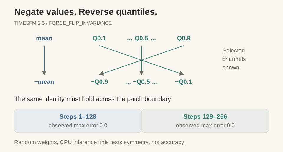
The model can enforce a symmetric result by combining predictions for x and -x, applying the channel transformation before averaging. That makes this a useful implementation property: the test does not need a trained model to determine the expected relationship between the two outputs.

It does need to reach every decoding branch that contributes to the forecast.

Why a 128-Step Test Is Too Short

The pinned 2.5 model definition specifies an output patch length of 128. A horizon of 256 reaches the continuation path. In the PyTorch decoding code, the sign-flipped pass applies flip_quantile_fn both to prefill output and to reshaped autoregressive output before concatenating them.

The accompanying regression test explains the historical failure: a missing quantile reversal in the continuation branch broke the identity after the first patch. I verified the corrected revision. I did not check out and execute the earlier broken revision, so the historical diagnosis comes from the upstream regression test, while the measurements below come from my run.

This is an example of choosing a test size from control flow. Doubling the horizon serves a specific purpose: it enters code that a shorter forecast never executes.

The CPU Run

I installed the pinned source and used PyTorch 2.8.0+cpu, NumPy 2.2.6, Python 3.12.8 and pytest 8.4.2 on Windows. The focused run included the sign-invariance test and the base utility tests:

python -m pytest tests/test_force_flip_invariance.py \
  tests/test_base_utils.py -q
17 passed in 11.51s

The invariance fixture initializes the actual 200M-class model with random weights and disables Torch compilation. It performs local CPU inference; it does not download pretrained weights or call a hosted service.

I then used a standalone probe to report errors separately on either side of the patch boundary. The input was a seeded, mixed-sign array with shape [1, 256], and the output had shape [1, 256, 10].

Forecast region	Maximum absolute symmetry error
Steps 1–128	0.0
Steps 129–256	0.0

The assertion allowed absolute and relative tolerance of 1e-4; the observed values were exactly zero in this run. That result verifies the configured algebraic relationship for this fixture. It is not a forecast-error metric.

The configuration matters. I enabled force_flip_invariance and disabled positivity inference, input normalization, quantile-crossing repair, backcast output and the continuous quantile head. In particular, clipping negative predictions because an input was classified as positive would interfere with the identity being tested. These switches keep the assertion about the symmetry path itself.

A Property Test Before an Accuracy Benchmark

Random weights cannot tell us whether the model predicts demand, prices or sensor readings well. They can reveal whether a postprocessing rule changes meaning halfway through the horizon. That makes this check useful before spending time on a pretrained evaluation.

For a new backend or export path, I would retain the same paired-input test and choose horizons just below, at and above each output boundary. I would test additional postprocessing combinations separately, with expectations appropriate to their semantics. Combining every option in one large benchmark would make a failing identity much harder to locate.

The informative coordinate here is step 129. It marks the first point where an apparently uniform forecast begins depending on a different branch of the implementation.